Regional Estimates of Household Poverty, Consumption Expenditure and Inequality in India
June 2023 | Shivakumar and Niranjan R.
I Introduction
Growth is the most critical factor in alleviating poverty and it has remained the most researched issue in the modern world. Sustained growth reduces poverty; the economic literature is firm on this point. Numerous cross-country studies (Kraay 2006, (Dollar and Kraay 2000, Chen and Ravallion 2000, (Lopez 2006) have concluded that the main determinant of poverty reduction is the pace of economic growth. However, it also appears that the relationship is reciprocal-poverty reduction is good for growth because it unleashes the productive power of the poor. Hence, the presence of poverty and inequality necessitates the augmenting of the growth process and become more balanced between regions. It is argued that growth and equity are contradictory. However, it must be recognized that there is no contradiction between the demand for equity and growth (Aggarwal 2001). The
Shivakumar, Guest Faculty, Department of Economics, Gulbarga University Kalaburagi, Post Graduate Centre, Halhalli (K) 585415, Bidar District, Karnataka, Email: shivactg1988@gmail.com
Niranjan R., Assistant Professor, Department of Studies and Research in Economics, Vijayanagara Sri Krishnadevaraya University, Ballari 583105, Karnataka, Email: niranjan@vskub.ac.in
social concern of the two can be handled together, sustaining and sustained by each other (Raza and Aggarwal 1982). For many decades, ‘growth with equity and social justice’ has remained on the development agenda of several developing countries.
Generally, the concept of poverty relates to socially perceived deprivation of financial well-being with respect to basic minimum needs. It is increasingly recognized that poverty is not a static concept, it is a dynamic multidimensional thought. People’s experience of poverty differs depending on the depth of their poverty, as well as whether they endure poverty over a period of time, thus experiencing persistent/chronic poverty (Hume and Shepherd 2003), which has implications both for their own life course as well as for intergenerational transmission of poverty (Harper, Marcus and Moore 2003).
Current debates on poverty in developing countries have been concerned with monetary or income poverty, as well as with multidimensional concepts of relative deprivation, such as well-being, vulnerability, capability and social exclusion. The definition and conceptualization of poverty have significant implications for understanding poverty and for the design of poverty reduction policies. In recent times, social exclusion has been regarded as dynamic and effective conceptual framework for analyzing the multiple dimensions, causes and consequences of poverty. It points to the ‘processes of impoverishment, structural characteristics of societies responsible for deprivation and group issues which tend to be neglected in other approaches’. In particular, the social exclusion approach is often contrasted with the monetary or income approach, which is most commonly used in policymaking. The monetary approach identifies poverty with the lack of sufficient income and it has been criticized for its narrow perception with physical needs while ignoring the structural causes of poverty.
In India, planned intervention in the poverty scenario can be traced back to the beginning of the planning period in the early 1950s. The government has not only worked for accelerating economic growth and development through five years plans, but it has also been implementing several anti-poverty schemes such as community development programs in 1952 to The National Rural Employment Guarantee Act in 2006 and also engaged poverty in a multidimensional aspect by focusing on social exclusion issues and integrating that with poverty, which is a theme of 11th five year plan, the inclusive growth and the same strategy is continued in the 12th five year plan as well. Despite all these developmental policies, according to the World Bank estimates in 2011, based on 2005’s Purchasing Power Parity (PPP) 23.6 per cent of Indian population or about 276 million people live below $1.25 per day. According to The United Nations Millennium Development Goals (MDG) programme, 270 million or 21.9 per cent people out of 1.2 billion populations live below the poverty line of $1.2 in 2011- 2012. This percentage of population is considered to be poor on an international criterion suggested by World Development Report (World Bank 2012). In October 2015, the World Bank updated the International Poverty Line (IPL) to $1.90 a day based on International Comparison Programme Purchasing Power Parity (PPP),
indicating the international equivalent of what $1.90 a day could buy in United States in 2011. The new IPL replaces the $1.25 per day figure, which used 2005 data. Recently, the Work Bank found that the global extreme poverty rate fell to
9.2 per cent in 2017, from 10.1 per cent in 2015. That means 689 million people are living on less than $1.90 a day and this 10.1 per cent fell from 11.2 per cent in 2013. At a larger poverty line, 24.1 per cent of the world’s people are living on less than $3.20 a day and 43.6 per cent on less than 5.50 per cent a day in 20171.
The earnest Planning Commission in 1979 estimated household poverty using Household Consumption Expenditure Data collected by the National Sample Survey Office (GOI 1979). It defines the poverty line, based on monthly per capita consumption expenditure (MPCE). The existing all India rural and urban poverty lines, in the per capita calorie norms of 2400 (rural) and 2100 (urban) were originally defined in terms of per capita total consumer expenditure at 1973-1974 market prices and adjusted over time across states for changes in prices. The all India poverty line so defined in 1973-1974 was ₹49.63 for rural areas and ₹56.64 for urban areas. The methodology for the estimation of poverty has been based on their commendations made by the Expert Group headed by Suresh D. Tendulkar which submitted its report on December 2009; according to it, the poverty lines at all India levels based on MPCE is ₹447 for rural areas and ₹579 for urban areas in 2004-2005. The all India poverty line for 2004-2005 adjusted for prices was
₹356.30 for rural areas and ₹538.60 for urban areas. For the year 2009-2010, the planning commission has defined the poverty line as ₹22.40 per capita per day in rural areas and ₹28.60 per capita per day in urban areas. This translates to ₹672.80 per capita per month in rural areas and ₹859.60 per capita per month in urban areas. Based on these cut-offs, the percentage of people living below the poverty line in the country has declined from 45.3 per cent in 1993-1994 to 37.2 per cent in 2004- 2005 and further declined to 29.8 per cent in 2009-2010. Even in absolute terms for the period 2004-2005 to 2009-2010, the number of poor people has fallen by
52.4 million. Of this, 48.1 million are rural poor and 4.3 million are urban poor. Thus, poverty has declined on an average by 1.5 percentage points per year between 2004-2005 and 2009-2010. Similarly, MPCE (at constant prices) has also increased from ₹558.78 and ₹1052.36 during 2004-2005 to ₹707.24 and ₹1359.75 in 2011-2012 in rural and urban areas respectively. The improvement in these social indicators is a reflection of a fall in deprivation. But ironically even after the elapse of seventy years after independence about one-third of our total population still suffers from abject poverty and a large section of poverty afflicted people is entangled by the poverty trap, i.e., they suffer from chronic poverty. The incidence as well as intensity of poverty, has also been reflected in its various dimensions, viz., the social, regional, occupational, ethnical, etc., in both rural and urban areas of our economy. Considerable attention was devoted in the past to analyzing poverty and social inequality in India at the national and state levels and also to devise state level plan allocations (Mishra and Joshi 1985) (Kurian 2000) (Gulati 1977). However much less is done at district or sub-regional levels, though the earnest Planning Commission has long back emphasized district level planning
(Aziz 1993). Meanwhile, the center of attention of much of the literature has been on vertical poverty and inequality, i.e., Inequalities across income or expenditure classes. In a plural society like India, with people of different castes and religions, it is equally important to focus on ‘horizontal inequalities’, i.e., disparity between different and certain identifiable social groups in the economy, at the state level and sub-regional level.
The important value addition of the study to the existing list of literature on household poverty is that it examines the extent, and intensity of household poverty and consumption expenditure covering two quinquennial rounds at regional level among socio-religious groups. The study makes use of various state- specific poverty lines based on the Tendulkar Methodology for both rural and urban sectors separately. The study covers 35 states into Six NSS regions2 classified by NSSO and compares the 61st (2004-2005) and 68th (2011-2012) rounds of NSSO Data. The rest of the paper is structured as follows. Section II introduces the poverty estimation methodologies in India, Section III presents a brief review of the literature, Section IV discusses data, methodology and econometric specification and identification, and Section V deals with a comprehensive empirical analysis of poverty in India. Finally, the last section concludes with policy implications.
II Poverty Estimation Methodology in India
In India, Dadabhai Naoroji was the first person to discuss the concept of poverty. After independence, there have been several efforts to develop mechanisms and methodologies to construct the poverty line and identify the number of poor in the country. In 1962, the Planning Commission3 constituted the working group to define the poverty line based on minimum calorie requirements suggested by the Indian Council for Medical Research (ICMR) which is 2,200 kl for rural and 2,100 kl for urban areas. The monetary value of these calories for a family of five people was fixed at ₹100 per month or ₹20 per capita, per month in 1960-1961 prices in urban areas.
In 1979 the Planning Commission constituted the Task Force Committee to estimate the percentage of population below the poverty line; the committee fixed 2400 kl per capita, per day in the rural area and 2100 kl per capita, per day in the urban area and estimated ₹49.09 and ₹56.64 monthly per capita for all India for both rural and urban sectors. Planning Commission (1984) did not re-define the estimation methodology of poverty, it adopted the methodology of the earlier task force committee, and accordingly fixed ₹89.50 and ₹115.65 as Monthly Per capita Consumption Expenditure (MPCE) for rural and urban area sectors as particularly. Estimates 45.65 per cent rural, 40.79 per cent of urban, and overall 44.48 per cent of the population is below the poverty line in India. Later in 2005, the Planning Commission constituted the expert group under the chairmanship of Suresh D. Tendulkar. The committee did not construct a poverty line but they espoused earlier expert group of Lakdawala methodology and the committee fixed ₹447 and
₹579 per capita per month consumption expenditure for both rural and urban sectors which is based on minimum calorie requirements as 2100 calorie for rural and 1776 calories for urban sector. The Rangarajan Committee (2012) computed the poverty level based on average requirements of calories of 2,155 kcal per person, per day, for rural areas and 2,090 kcal per person, per day, for urban areas4. According to the estimates of Rangarajan, there are 30.9 per cent (260.5 million poor people) in the rural area and 26.4 per cent (102.5 million poor people) of the population is below the poverty line in urban areas and overall 29.5 per cent (363 million people) at all India level of population is poor.
III Literature Review
Many scholars examined the distributional aspects of household poverty and consumer expenditure. Moreover, the inadequacy of data on households and increasing interest in the size distribution of income and inequality has made the researchers rely heavily on sample surveys, especially those conducted by NSS. Mehtabul (2009) in his study examined the differences in welfare, as measured by Per Capita Income across the social groups in rural India by using NSS household consumption expenditure of the 61st round (2004-2005). The study reveals Scheduled Tribes households are most deprived in income existing across the entire welfare distribution followed by SC and OBC with respect to general category households. The study suggests that government policies must raise the human capital and increase effective assets of the SC and ST households especially in the rural sector. Panagariya and Mukim (2013) provided a comprehensive analysis of poverty for 17 larger states in the country, by estimating poverty (headcount ratio) for rural and urban sector and for socio-religious groups by using two official poverty lines based on Lakdawala and Tendulkar Methodology. The study, during 1993-1994 and 2009-2010, found poverty declining for various social and religious groups in all the states, secondly the reduction of poverty is larger in scheduled caste and scheduled tribes than the other backward class. Gupta and Mishra (2014) in their study examined food consumption pattern across selected social and economic groups and identified food consumption regions in India. The study was also done to show determinants of food item wise consumption pattern in the rural sector in India. The study argues that, such disaggregated measures bring out the multiplicity in food consumption patterns and helps identifying the socio-economic groups suffering from deprivation in food consumption. Arora and Singh (2015) by using unit level NSSO household consumption expenditure data of 61st (2004-2005) and 68th (2011-2012) round, estimated regional as well as disaggregated levels of poverty for socio-religious groups, for both rural and urban sector of Uttar Pradesh (UP). The study classified the state into different regions and identified critical poverty affected regions in UP across socio-religious groups. The study also made use of logistic regression to identify the determining factors of poverty and found the level of poverty across the central region, southern region and eastern region is unfairly distributed.
Sumedha and Meenakshi (2015) in their study, measured the link between inequality in physical infrastructure in 17 major states in India, both rural and urban sectors, by using the household consumption expenditure survey of 38th (1983), 50th (1987-1988), 61st (2004-2005) and 66th (2009-2010) round of NSSO
respectively. The study also measured Inequality in per capita net state domestic product (NSDP) by using the Gini coefficient and it shows the impact of infrastructure on consumption inequality across the states. Datt, Gaurav, Martin Ravallion and Rinku Murgai (2016) by using a newly constructed dataset of poverty estimates for India and covering 60 years, including 20 years since the economic reforms of 1991. The study found that, acceleration of poverty declined since 1991, in spite of the rising inequality. Post-1991, growth was at least as pro- poor as in the previous decades and growth in the secondary and tertiary sectors of the economy, drove the bulk of the post-1991 poverty to decline in the urban sector. Roy (2017) in his study examined the status of hunger across major states of India, by conceptualizing it in terms of calorie under-nourishment. The study also estimated multivariate analysis in the form of logistic regression to explore the determinants of hunger and found that it was negatively and significantly influenced by per-capita food grain production, while it was positively and significantly affected by poverty, price level, and economic growth. Maitra and Menon (2019) measure the pattern and correlate excess weight of adults in India by using panel data. In their study they found urban women are predominantly at risk of being overweight and income or wealth, comparative inequality and lifestyle choices strongly correlated with body mass index. Balasubramaniam, Divya, S. Chatterjee and B. David Mustard (2019) measure the relationship among access to drinking water, sanitation facility and health outcomes for children in India by using NFHS 20015-2006 household survey data to construct nutritional distribution and health measures for children ages of below 2 years. By estimating regressions approach, they found public goods such as piped water are not associated with improving child health outcomes. Further rural children at the lower nourishing distribution, benefit much more than urban children. Especially in rural areas, children are progressive evidence against ‘one-size-fits-all’ policies, private sanitation and mother education and for children in the middle of the restrictive nutritional distribution.
There exist several studies on assessments and determinants of poverty, both at macro and micro level, inter-regional studies focusing on spatial divergence in poverty. Most of the empirical works on poverty and inequality are examined through regional disparity. However, with respect to India, there are a few empirical studies focusing on regional poverty and inequality within the state and linking the same to poverty and inequality. However, the empirical analyses on poverty and consumption expenditure focusing on regional level across socio- religious groups are merged. The current study with respect to India fills this gap, by analysis of the regional level across socio-religious groups in the country.
IV Data and Methodology
The study estimates household poverty at regional level, across socio-religious groups for various NSS regions by 61st and 68th rounds of MPCE data surveyed by National Sample Survey Organization. The study compares 61st and 68th round of quinquennial surveys, based on this comparison of two surveys, the poverty levels are compared to Six NSS regions classified by National Sample Survey Office, i.e., Northern Region5, Central Region6, Eastern Region7, North Eastern Region8, Western Region9 and Southern Region10 states in the country. NSS provides monthly per-capita expenditure data for three reference periods: Uniform Recall Period (URP), Mixed Recall Period (MRP), and Modified Mixed Reference Period (MMRP)11The URP or MRP-based consumption data are available in the 61st Round in 2004–2005, the 66th Round in 2009–2010, and the 68th Round in 2011– 2012. On the other hand, MMRP-based consumption data are available only in the 66th and 68th NSS Rounds. Only the 61st Round and 68th Round data are considered by taking MRP-based consumption expenditure data, as MRP-based estimates capture the household poverty and consumption expenditure of poor households on low-frequency items of purchase more satisfactorily than does the URP data.
The study using MPCE of MRP to measures incidence of mean poverty, i.e., Head Count Ratio (Hp): which is measured as the “Percentage of population which is below the poverty line.
● Head Count Ratio (Hp): The number of poor estimated as the proportion of people below the poverty line is known as Head Count Ratio and it is calculated by dividing the number of people below the poverty line, by the total population.
Hp= n
N
…(1)
Hp = Headcount ratio, n = Number of people below poverty line and N = Total population. For estimating the household poverty, the study makes use of state wise specific poverty line, based on Tendulkar Methodology for rural and urban sectorsseparately12. In addition, the study used binomial Logit or Probit regression model since it is an appropriate technique to observe the likelihood of a household for being poor or a risk of the household on entering or escaping poverty. The study also measures household MPCE and consumption inequality by using Gini coefficient and Lorenz curves for estimating Income/consumption inequality at regional level across socio-religious groups in India.
● Gini Coefficient: It is used to measure inequality, in income or wealth distribution among a population. The Lorenz curve is a graphical representation of inequality developed by American economist Max Lorenz in 1905. The Gini Ratio lies between 0 to 1, 0 represents perfect income equality and 1represents perfect income inequality
Formally, the Lorenz curve can be expressed, as let in xi be a point on the X-axis, and yi a point on the Y-axis. Then
𝐺𝑖𝑛𝑖 = 1 − ∑N (𝑥i − 𝑥i–1)(𝑥i + 𝑥i–1) …(2)
The National Sample Survey of “Consumer Expenditure” (Schedule 1.0) was conducted in the 61st Round in 2004–2005, considering 124,644 sample households in India (79,298 in rural areas and 45,346 in urban areas), which represent 609,736 persons/individuals total (403,207 in rural areas and 206,529 in urban areas). On the other hand, the NSS of ‘Consumer Expenditure’ (Schedule1.0, Type 1) in the 68th Round, 2011–2012 was surveyed by considering 101,662 households (59,695 in rural areas and 41,967 in urban areas), which consist of 464,960 individuals/persons (285,796 in rural areas and 179,164 in urban areas). The average Monthly Per capita Consumption Expenditure (MPCE) of 2004-2005 in current prices was ₹579 and ₹1105, in rural and urban areas, respectively. On the other hand, the average MPCE of 2011-2012 in current prices was ₹1287 and ₹2477, in rural and urban areas respectively (Tripathi Sabyasachi 2018). Due to unavailability of recent NSSO survey of household MPCE data, the study is limited to only 61st and 68th rounds.
V Household Poverty in India: Empirical Analysis
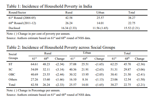
Table 1 reveals that rural poverty is higher compared to urban poverty in India. The study found that, 42.58 per cent of rural households are poor, which is
higher than 25.57 per cent of urban poverty in 2004-2005. Meanwhile, in 2011- 2012, the rural poverty it came down to 26.24 per cent and the urban poverty declined to 14.01 per cent. As a country as a whole, the household poverty declined by 15.52 per cent for the period from 2004-2005 to 2011-2012.
Table 2 brings out social group wise household poverty; the results in the table show that, between 61st and 68th round, poverty declined across various social groups. The study found higher poverty in scheduled tribes and scheduled caste than the OBC and others in the country. During the period, poverty decline is highest among the scheduled caste, is 3.06 points per annum followed by OBC which is 2.41 points per annum, scheduled tribes is 2.36 points per annum and others is only 1.50 points per annum, for both rural and urban sector.
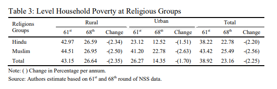
Table 3 shows that among the religious groups, where Muslim households are comparatively poorer in the country compared to Hindus, it has been noted that, Muslims are also significantly deprived educationally and marginalized occupationally. In the 61st round, the study found Muslim households have higher poverty by 43.42 per cent whereas the level of poverty among Hindu households is 38.22 per cent. Meanwhile, in 68th round as well, higher household poverty is found in Muslims households to the tune of 25.49 per cent, compared to Hindu households of 22.78 per cent, for both rural and urban sector.
The National level poverty has been illustrated by the author for 61st (2004- 2005) and 68th (2011-2012) round and it is mapped separately in the below Figures 1 and 2.
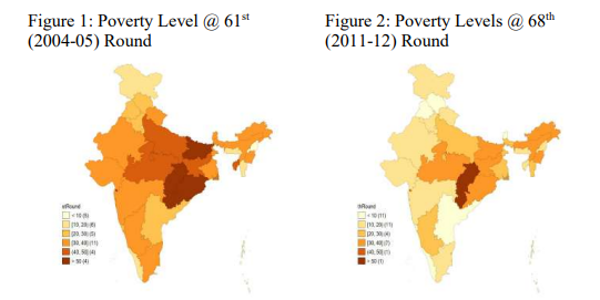
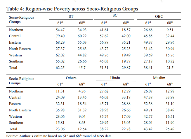
Table 4, presents NSS region and socio-religious group-wise levels of poverty in India. The results reveal that higher levels of household poverty among socio-religious groups are particularly found in districts of North Eastern, Central and Western region. Meanwhile, comparatively lower levels of household poverty is found in Western, Northern and Southern region states, for both rural and urban sector, during the study period 2004-2005 to 2011-2012.
II Logistic Regression
Poverty determinants are usually estimated by using Probit or Logit model. In Probit or Logit model13, dichotomous variables are used which represents whether a household is poor or not. This dichotomous variable is regressed on a set of supposed explanatory variables like region, educational level, asset ownership, household size, religious groups, occupation and composition of households etc. Specifically, certain explanatory variables could be identified which are significantly associated with being poor or non-poor (Baulch and McCulloch 1998). In this study, the Logit model was used to find the determinants of rural poverty with the help of poverty status. The Logit or Probit regression model is the appropriate technique to observe the likelihood of a household for being poor or non-poor. To identify key determinants of poverty we first computed a dichotomous variable indicating whether the household is poor or not. That is,
Poor= 1, if household is poor 0, if household non-poor
A Logistic regression model is a univariate binary model. For dependent variable Yi, there are only two values one and zero, and a continuous independent variable Xi, that
Pr (Yi=1) = F (x’ib) …(3)
Here b is a parameter that needs to be estimated and F is logistic cdf. The basic formula application of Logit model is:
𝑃1 = 𝐹 (𝛼 + 𝛽𝑥𝑖) = 1
[1+e—(α+ βxi)]
…(4)
Where xi is the probability that ith households will be poor given Yi, where 𝛼 is a vector of explanatory variables. e is the base of natural logarithm. Equation 5 can be written as:
𝑃𝑖 [1 + 𝑒–(α+βxi)] = 1 𝑂𝑟 …(5)
| Pi |
𝛼 + 𝛽𝑥𝑖 = 𝑙𝑜𝑔 ( ) …(6)
1–Pi
The ration ( Pi ) is called the log odd or Logit, which acts as the dependent
1–Pi
variable
This ratio will give the odds of a household, whether it is poor or not. A positive sign of estimated coefficients would mean that the probability of being
poor is higher than reference category and vice versa keeping all other characteristics constant. Putting it another way “A number greater than one of log odds indicates a positive association between independent and dependent variable, while a number between Zero and one indicates negative association among both” (Hoffmann and P. Johan 2004). In equation 6, the coefficient gives the change in log odds of the dependent variable, not the changes in the dependent variable itself. Therefore, to make the interpretation straightforward, a logistic can be converted to the odds ration, using exponential function (Joshi N.P. 2012). The functional form of odds ratio can be given as equation
𝑂𝑑𝑑𝑠𝑟𝑎𝑡𝑖𝑜 = [ pi ] = 𝑒α+β1K1i+β2K2i+β3K3i…+βnKni+si …(7)
1–pi
Here, the odds ratio is simply the ratio of the probability that the household will be poor to the probability that the household will be non-poor. In case of binary independent variables, exponential of the respective coefficient, gives the proportion of change odds for shift in the given independent variable. However, if the independent variable is continuous exponential of coefficient, it is associated with the effect of per unit change in the given independent variable to the odds ratio. In both type of variables, the sign of coefficient reveals the direction of change.
Empirical results based on the estimation of econometric model and trend in household poverty head counts, the main objective of the econometric model was to determine the factor affecting poverty status in the country (Hashmi A. 2008).
The Particulars of the Regression are as Follows
- Dependent variable – A dummy variable called poor is created, which takes the value’ l’ if the individual is poor and the value ‘0’ if he or she is non- poor.
- Independent variables – Sector, Social Groups, Religious Groups, Age, Regional Level, Education Level, Household Occupation and Land poses/holding.
The final model applied is as below:
Logit (Zi) = α+ β1X1+ β2X2+ β3X3+ β4X4+ β5X5+ β6X6+β7X7+ β8X8 …(8)
Where:
X1= Sector, X2=Social Groups,
X3=Religious Groups, X4= age, X5=Regional Level, X6= Education Level,
X7= Household Occupation and X8=Land poses/holding.
This logistic regression equation was arrived at, using a forward stepwise selection method. Using the data, the logistic regression has been estimated to determine the factors affecting poverty in India. Below table 5, exhibits that the probability of a household being poor in urban sector is an almost equal probability of falling under poverty to the (Rural) reference group.
Among the social groups, the Scheduled Caste and OBC category being poor were compared to the reference group of Scheduled Tribes but the other category households have low probabilities of falling under poverty, this results is evidenced for both the rounds. The Muslim household is also found to have higher poverty and the same is statistically significant at one per cent, for both 61st and 68th rounds.
The household size also has strong positive relationship with the poverty status, as well the household occupation in both 61st and 68th rounds. The male and female adults, aged between 19 to 30 years and 31 to 45 years have strong positive relations with poverty status. The study also shows, the NSS region-wise levels of poverty, wherein the households of Central, Eastern and North Eastern Regions in 2004-2005 have higher probability of falling under poverty, in comparison to the reference region – the Northern region. However, in relation to 61st round estimates the probability of households falling under poverty, during 68th round have shot-up in Central (3.3947), Eastern (2.578) and North Eastern (3.14) region. Similarly, during the same period the probability levels of household poverty declined in western (1.56) and southern regions (0.9217). In addition, in 68th round compared to the reference region the probability levels of household poverty is significantly higher in Central, Eastern, North Eastern regions and it is lower in southern regions.
The education variable also showed a significant positive correlation with poverty status. The levels of education is a vital factor, which influences the chance of being poor and non-poor, and there is less chance to falling under poverty if the household head has primary-secondary and higher levels of education. Another important aspect of these results is that the basic education has a strongly negative impact on poverty status; however, the extent of poverty for below primary level of education, is greater and statistically significant.
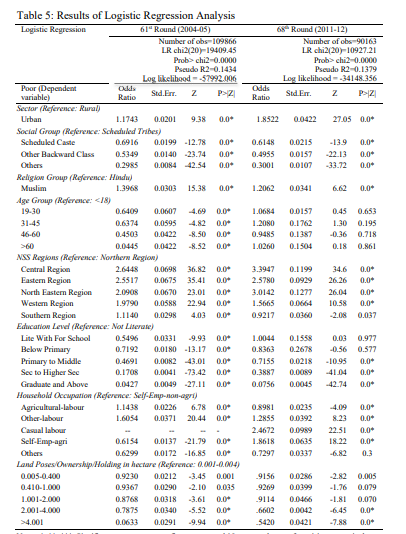
However, the likelihood of being poor is more for a household head being an agricultural and other labor (household occupation). There was higher chance of being poor for a household if they agricultural and casual labors. The land holding or ownership also shows significant positive relationship with poverty. The land holding is one of the important determining factors of poverty, lower the land holding, there will higher the probability of being poor in rural sector.
II Monthly Per-Capita Consumption Expenditure (MPCE) in India
Consumption is an important activity performed by the household sector and it has always been a strong and major driver of growth in the economy and it is the most important component of GDP. The study intended to examine the level of household monthly per-capita consumption expenditure, sector wise and regional level among social groups in India.
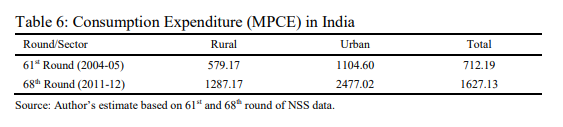
The study also estimates household average monthly per-capita consumption expenditure of 61st and 68th rounds, for both rural and urban sectors separately. The Table 6 reveals the lower MPCE found in 61st round is ₹712.19 of both rural (₹579.17) and urban sector (₹1104.60). In 68th round it has increased in double proportion to ₹1627.13 of rural (₹1287.17) and urban (₹2477.01) sector respectively.
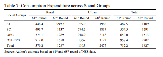
Table 7 study estimated household monthly per capita consumption expenditure among the social groups for rural and urban sector separately. In 61st round, the average monthly per capita consumption expenditure is low in among Scheduled Tribes households with ₹487.5 followed by Scheduled Caste -₹554.5 and OBC – ₹650, but the other category households have a higher consumption
expenditure of ₹958.4 per month. Meanwhile, in 68th round the MPCE has increased among all the social groups. However, lower MPCE is found among ST households with ₹1109/month followed by SC households -₹1291, the OBC households have ₹1513 and other households have higher the MPCE of ₹2202 respectively.
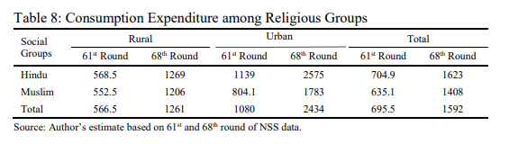
Table 8 shows that, among the religious groups, Muslim households have comparatively lower MPCE than the Hindu households for both 61st and 68th rounds. In 61st round, the Muslim households have the MPCE of ₹635.1/month and Hindu households’ MPCE is ₹704.9. Similarly, in 68th round, the MPCE among the Muslim households is ₹1408 and the Hindu households’ is of ₹1623 respectively.
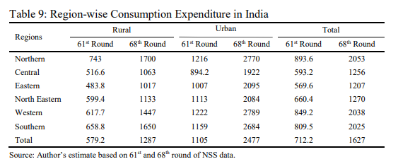
The study estimates household MPCE among the NSS regions for both 61st and 68th round separately. Table 9 reveals that in 61st round lower MPCE is found in the states of Eastern region with ₹569.6, Central region is ₹593.2 and North Eastern is ₹660.4 and higher MPCE of the households is found in Northern region which is ₹893.6, Western region is ₹849.2 and Southern region is ₹809.5. Meanwhile, in 68th round the MPCE increased in all regions. Whereas, lower MPCE is found in Eastern region with ₹1207, Central region is of ₹1256 and North Eastern is ₹1256.
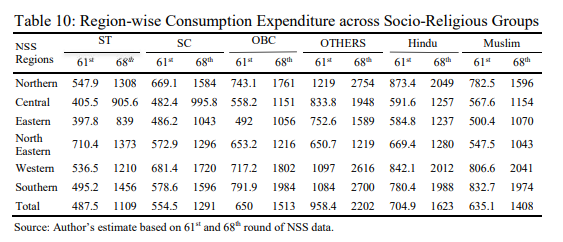
The study also estimates household level MPCE across socio-religious groups among the regions shown in table 10. The table 10 highlights the, significant distribution of MPCE among the socio-religious groups for both 61st and 68th rounds. In 61st round, all the socio-religious groups are found to have lower MPCE and in 68th round, the mean consumption expenditure increased significantly.
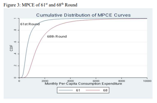
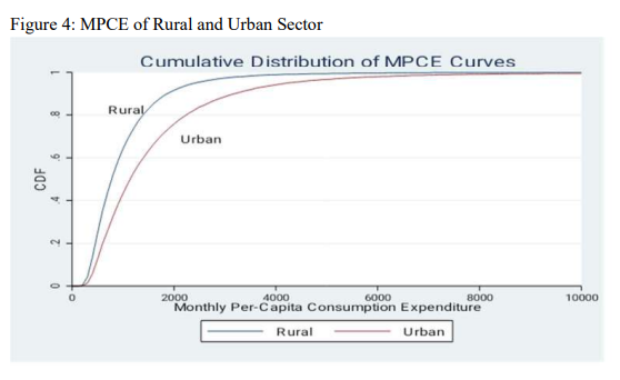
In addition, the study measures cumulative distribution of Monthly Per- Capita Consumption Expenditure (MPCE) across the classes to estimate the consumption inequality. Figure 3 and 4 compares the cumulative distribution functions (CDFs) of MPCE for the 61st (2004-2005) and 68th (2011-2012) round for both rural and urban sectors. It is apparent that the 61stround has higher MPCE compared to the 68th round and the rural sector has higher MPCE compared to the urban sector, in both the 61stand 68th round of the consumption expenditure.
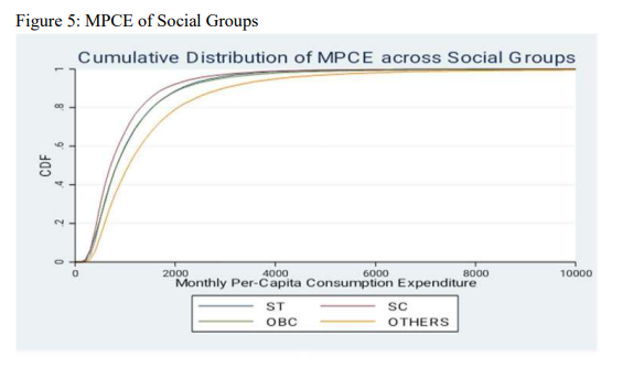
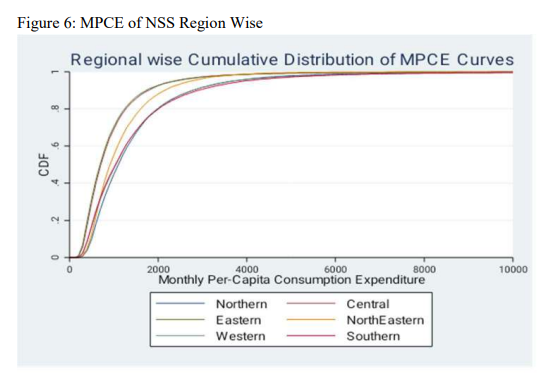
Meanwhile, Figure 5 exhibits cumulative consumption distribution function across social groups. It is noticed that there is a larger monthly per capita consumption by SC, ST and Other Backward Class (OBC) in the early stages and thereafter a deviation can be noticed across the social groups. Figure 6, exhibits cumulative consumption distribution function across NSS regions of India; it is observed that there is higher monthly per capita consumption in Northern and Central regions followed by North Eastern, Eastern, Western and Southern regions.
II Inequality in Household Consumption Expenditure
The following tables and figures exhibit the inequality measured through Gini index and Lorenz Curve of Monthly Per Capita Consumption Expenditure of 61stand 68th round, for both rural and urban sector. Table 11 shows inequality values, the results reveal that there is no significant difference between in MPCE between the rounds but they deviate towards the end. The Gini value of 61st round is 0.340 and the Gini value of 68th round is 0.355 but they deviate at the end. Whereas, in case of the Lorenz curve of MPCE of both 61st (2004-2005) and 68th (2011-2012) rounds; it reveals that in 61stround, Lorenz curve is closer to the 45º line, the line of equality, and that the 68thround signifies lesser inequality in MPCE (Figure 7).
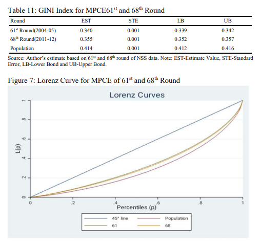
The Lorenz curve has been used for several decades, being the most popular graphical tool for visualizing and comparing income inequality and it provides complete information on the whole distribution of incomes relative to the mean (Doclos Jean-Yves and Araar Abdelkrim 2009).
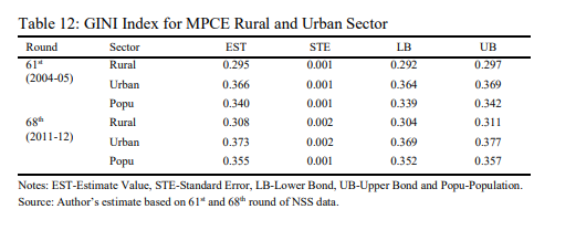
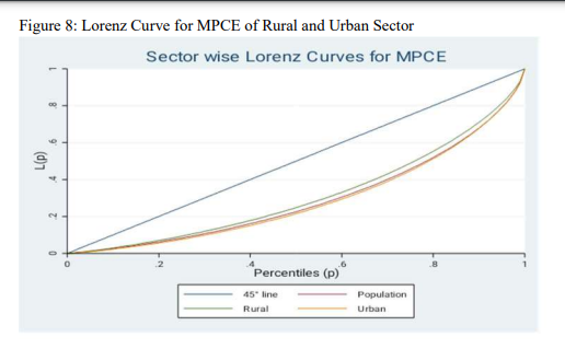
The Gini index value indicates a significant deviation between the rural and urban sector MPCE. The table 12 expresses a lesser inequality of consumption distribution for both 61stand 68th round. In 61stround, the Gini value for rural sector is 0.295 and urban sector is 0.366. Whereas, in 68th round the Gini value indicates larger inequality in consumption distribution with gini value of 0.308 for rural sector and 0.355 for urban sector, the Lorenz curve also reveals, the rural sector Lorenz curve is closer to the 45º line, the line of equality, and the urban sector signifies lesser inequality in MPCE (Figure 8) for both 61st and 68th rounds.
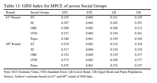
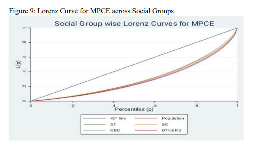
The inequality index of MPCE across social groups is shown in above table 13, that exhibits significant inequality in household consumption expenditure in both 61st and 68th rounds for scheduled tribes (ST), scheduled cast (SC), other backward castes (OBC) and others in the country. In 61st round, the consumption inequality is larger among the others with Gini index value of 0.357 followed by ST with Gini value 0.325, OBC with Gini value 0.309 and SC is lower with Gini value 0.287. Whereas, in 68th round, higher consumption inequality is found in others households with Gini value 0.373 followed by OBC with Gini value 0.333, ST with Gini value 0.319 and lastly SC with a Gini value of 0.317. Meanwhile, Figure 9 reveals Lorenz curve across social groups where for scheduled tribes it is closer to the 45º line and the rest of respective caste (SC, OBC and Others) signifies lesser inequality in MPCE for both 61st and 68th rounds.
The study also estimates Gini Index among the religious groups in the country. Table 14 shows that, in 61st round, larger consumption inequality is found in Hindu households with Gini value of 0.342 and Muslim households have lower inequality with a Gini value of 0.306.
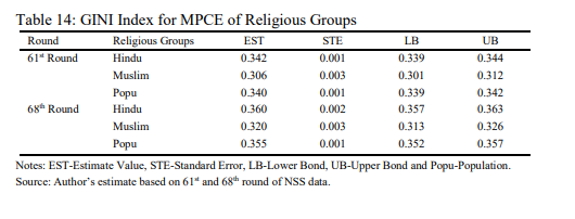
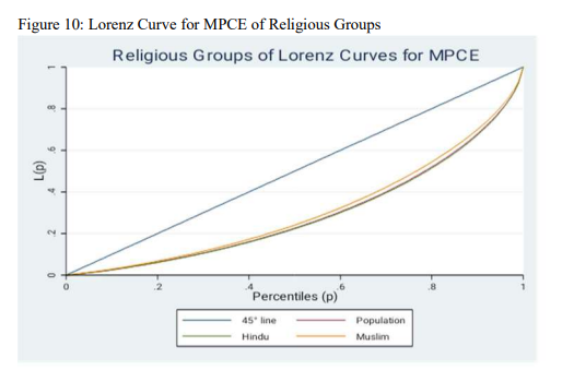
Meanwhile, in 68th round, higher consumption inequality is found again in Hindu households with Gini value of 0.360 as compared to Muslim households with Gini value of 0.320. Meanwhile, Figure 10 also reveals that among religious groups, the Lorenz curve of Muslims households closer to the 45º line.
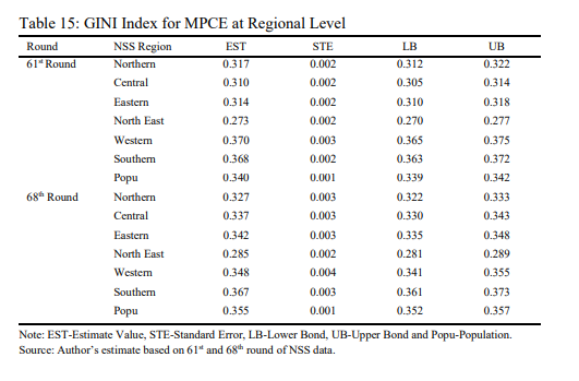
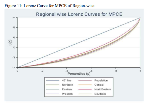
The study examined the extent of intensity of MPCE inequality across NSS regions in the country (above Table 15). The country has six NSS regions (classified by NSSO), in 61st round. Among the six regions, the Western region consists of five states, that were found higher inequality in MPCE (0.370) which is above the country average with a Gini value of 0.340, followed by Southern region with a Gini value of 0.368, Northern region with a Gini value of 0.317, Eastern region with a Gini value of 0.314 and Central region with a Gini vale of 0.310; their regions are below the country average in-terms of MPCE. There is no significant difference between Eastern and Central regions and lastly North Eastern region has a lower household consumption inequality in the country, with a Gini value of 0.273 for both rural and urban sector. Meanwhile, in 68th round, a larger consumption inequality is found in Southern region, with a Gini value of 0.367, followed by Western region with a Gini value of 0.348, Eastern region states with Gini value of 0.342, Central region with Gini value of 0.337 and Northern region with Gini value of 0.327. However, the inequality in North Eastern region states is lower with a Gini value of 0.285 respectively. Meanwhile, the movements of Gini values are exhibits in Lorenz curves, which shows 61stand 68throunds of consumption expenditure among the NSS regions in Figure 11. Among the regions, that figure exhibits where Northern region Lorenz curve is closer to the 45º line compared to the rest of the regions.
II Conclusion and Policy Implications
Poverty is one of the most serious issues being faced by any country. It is measured in terms of a specified normative poverty line, reflecting the minimum living standard of people. The current study estimates the regional level of household poverty and inequality in India.
The results reveal that the incidence of household poverty is higher with 38.27 per cent and lower MPCE with ₹712.19 in 61st (2004-2005) round and lower levels of poverty with 22.75 per cent and higher MPCE ₹1104.60 is found in 68th (2011- 2012) round. Meanwhile, among the socio-religious groups, higher levels of household poverty are found among the Scheduled Tribes and Scheduled Caste which are larger than OBC and Others and also Muslim households are comparatively poorer than Hindus between the rounds but they deviate towards the end.
Finally, this study identified the factor responsible for pathways out and in, among socio-religious groups household or associated with poverty and consumption expenditure status. A logistic regression model is estimated with an extensive range of household characteristics to discover the determinants of household poverty. The results show lack of household education, occupation and low levels of landholdings as the major determinants of poverty. The probability of being poor decreased with a lower household size and higher land holdings.
Despite various policies to alleviate poverty, malnourishment, illiteracy, hunger and lack of basic amenities continue to be a common feature in some of the regions and social groups in the Country. The policy implementations should focus on development of educational infrastructure and self-employment programs in general; amongst rural households, with special emphasis on Scheduled Caste and Scheduled Tribe (ST) in the region. To contain spatial variation in poverty and inequality, the study suggests the improving of infrastructure in agricultural sector, which in turn increases income generation in the poverty-affiliated regions.
Endnotes
1. https://www.worldbank.org/en/topic/poverty/overview
2. Northern, Central, Eastern, North-Eastern, Western and Southern Regions.
3. 65-year old Planning Commission has been dissolved and a new institution name NITI (National Institution for Transforming India) Aayog has been constituted by the National Democratic Alliance (NDA) government in 1st January 2015.
4. Rangarajan Committee (2012), Methodology for Estimation of Poverty, Planning Commission, Government of India Report http://planningcommission.nic.in/reports/genrep/pov_rep0707.pdf
5. Northern Region consists of 7 States, i.e., Jammu & Kashmir, Himachal Pradesh, Punjab, Chandigarh, Haryana, Delhi and Rajasthan.
6. Central Region consists of 4 States, i.e., Uttarakhand, Uttar Pradesh, Chhattisgarh and Madhya Pradesh.
7. Eastern Region consists of 4 States, i.e., Bihar, West Bengal, Jharkhand and Orissa.
8. North Eastern Region consists of 8 States, i.e., Sikkim, Arunachal Pradesh, Nagaland, Manipur, Mizoram, Tripura, Meghalaya and Assam.
9. Western Region consists of 5 States, i.e., Gujarat, Daman & Diu, Dadra & Nagar Haveli, Maharashtra and Goa.
10. Southern Region consists of 7 States, i.e., Andhra Pradesh, Karnataka. Lakshadweep, Kerala, Tamil Nadu, Pondicherry and Andaman & Nicobar Island.
11. The Uniform Recall Period (URP) refers to consumption expenditure data collected using the 30-day Recall or reference Period. The Mixed Recall Period (MRP) refers to consumption expenditure data collected using the one-year Recall Period for five non-food items (i.e., clothing, footwear, durable goods, education, and institutional medical expenses) and 30-day Recall Period for all the rest of the items purchased. The Modified Mixed Reference Period (MMRP) refers to consumption expenditure data collected using the 7-day Recall Period for edible oils, eggs, fish and meat, vegetables, fruits, spices, beverages, refreshments, processed food, pans, tobacco, and intoxicants, and for all other items, the reference Periods used are the same as in the case of the MRP
12. http://planningcommission.nic.in/reports/genrep/pov_rep0707.pdf
13. A binary logistic regression model is considered the most appropriate model for the econometric analysis when dependent variable is dichotomous (binary) variable such as incidence of poverty in our case. It fits well for both continuous as well as categorical independent variables.
References
Aggrawal, Y. (2001), Disparities in Education Development, National University of Educational Planninf and Administration (NUEPA).
Ahluwalia, M.S. (1978), Rural Poverty and Agricultural Performance in India, Journal of Development Studies, 14(3): 298-323.
Almas, Ingvild, Anders Kjelsrud and Rohini Somanathan (2013), The Measurement of Poverty in India – A Structural Approach, Working Paper Norwegian School of Economics and Business Administration and University of Oslo, Bergen.
Arora, A. and P.S. Singh (2015), Poverty across Social and Religious Groups in Uttar Pradesh an Interregional Analysis, Economic and Political Weekly, L(52): 100-109.
Atkinson, A.B. (1983), The Economics of Inequality, Clarendon Press, Oxford.
———- (1987), On the Measurement of Poverty, The Econometric Society, 55(4): 749-764, https://www/jstor.org/stable/1911028
Aziz, A. (1993), De Centralized Planning: The Karnataka Experiment, New Delhi: Sage Publication. Balasubramaniam, Divya, Santanu Chatterjee and B. David Mustard (2019), Public Versus Private
Investment in Determining Child Health Outcomes: Evidence from India, Arthaniti: Journal of Economic Theory and Practice, 19(1): 28–60, https://doi.org/10.1177/0976747919854257
Baluch, Bob and N. McCullough (1998), Being Poor and Becoming Poor: Poverty Status and Poverty Transition in Rural Pakistan, IDS Working Paper 79.
Chen, S. and M. Ravallion (2000), How Did the Worlds’ Poorest Fare in the 1990s, World Bank.
Datt, Gaurav, Martin Ravallion and Rinku Murgai (2016), Four Questions and Answers on Growth and Poverty Reduction in India, Arthaniti: Journal of Economic Theory and Practice,15(12): 1–10, December, https://doi.org/10.1177/0976747920160201
Deaton, Angus and Jean Dreze (2002), Poverty and Inequality in India: A Re-Examination,
Economic and Political Weekly,37(36): 3729-3748, September.
Dev, M.S. (2018), Inequality, Employment and Public Policy, Indira Gandhi Institute of Development Research, Mumbai, WP-2018-003, pp. 1-53.
Doclos, Jean-Yves and Araar Abdelkrim (2009), Testing for Pro-Poorness of Growth, with an Application to Mexico, Review of Income and Wealth, 55(4): 853-881, December.
Dollar, David (2007), Poverty, Inequality and Social Disparities during China’s Economic Reform, World Bank Policy Research Working Paper 4253, June.
Dollar, David and A. Kraay (2000), Growth in Good for the Poor, Journal of Economic Growth,
7(3): 195-225.
Foster, Greer and E. Thorbecke (1984), A Class of Decomposable Poverty Measures, The Econometric Society, 52(3): 761-766, http://www.jstor.org/stable/1913475
Government of India (1979), Report of the Task Force on Projections of Minimum Needs and Effective Consumption Demand, Perspective Planning Division, Planning Commission, New Delhi.
———- (2014), Methodology for Estimation of Poverty 2014 Report, Planning Commission, http://planningcommission.nic.in/reports/genrep/pov_rep0707.pdf
———- (2019), Economic Survey Report (2018-19).
Gulati, S.C. (1977), Dimensions of Inter-District Disparities, Indian Journal of Regional Science,
9(2): 97-106.
Gupta, Abha and Deepak K. Mishra (2014), Food Consumption Pattern in Rural India: A Regional Perspective, Journal of Economic and Social Development, 10(01): 01-17.
Harpaer, C., R. Marcus and K. Moore (2003), Enduring Poverty and the Condition of Childhood: Life Course and Intergenerational Poverty Transmissions, World Development, 31(3): 535- 554.
Hashmi, A. Amara, Maqbool H. Sail and Maaida H. Hashmi (2008), Trends and Determinants of Rural Poverty: A Logistic Regression Analysis of Selected Districts of Punjab, The Pakistan Development Review, 47(4 Part II): 909–923.
Himanshu (2010), Towards New Poverty Line for India, Economic and Political Weekly, XLV(1): 38-48.
———- (2013), Poverty and Food Security in India, ADB Economics Working Paper Series No.369. Hoffman, Johan P. (2004), Germanized Linear Models: An Applied Approach, Boston/New York/
San Francisco, https://www.worldbank.org/en/topic/poverty/overview
Hulme, D. and Shepherd (2003), Chronic Poverty and Development Policy, World Development,
31(3): 399-402.
Jha, Raghbendra (2000), Reducing Poverty and Inequality in India: Has Liberalization Helped?
Working Paper No. 204 (UNU/WIDER).
Joshi, N.P. (2012), Determinants of Income and Consumption Poverty in Far-Western Rural Hills of Nepal – A Binary Logistic Regression Analysis, Journal of Contemporary India Studies: Space and Society, Hiroshima University, 2: 51-61.
Kraay, A. (2006), When is Growth Pro-Poor? Evidence from a Panel of Countries, Journal of Development Economics, 80: 198-227.
Kurian, J.N. (2000) Widening Regional Disparities in India: Some Indicators, Economic and Political Weekly, 35(7): 538-550.
Lopez, H. (2006), Dis Growth become Less Pro-Poor in the 1990s? Working Paper 3931, Washington DC: World Bank.
Maitra, Pushkar and Nidhiya Menon (2019), Portliness Amidst Poverty: Evidence from India, Arthaniti: Journal of Economic Theory and Practice, 18(2): 138–170, https://doi.org/10.1177/ 0976747918807005.
Mehtabul, A. (2009), A Distributional Analysis of Social Group Inequality in Rural India, IZA Discussion Paper No. 3973, January.
Mishra, G.P. and A. Joshi (1985), Regional Structure of Development and Growth in India (Vol. I and II), New Delhi: Ashish Publishing House.
Murgai, Rinku, M.H. Suryanarayana and Salman Zaidi (2003), Measuring Poverty in Karnataka the Regional Dimension, Economic and Political Weekly, 38(4): 404-408.
Pal and Ghosh (2007), Inequality in India: A Survey of Recent Trends, DESA Working Paper No.
45, ST/ESA/2007/DWP/45, pp. 1-28, https://www.researchgate.net/publication/23694225 Panagariya, A. and M. Mukim (2013), A Comprehensive Analysis of Poverty in India, Working
Paper No. 2013-01.
Rangarajan Committee (2012), Methodology for Estimation of Poverty Report, Planning Commission, Government of India, http://planningcommission.nic.in/reports/genrep/pov_rep 0707.pdf
Rangarajan, C. and S. Mahendra Dev (2014), Counting the Poor: Measurement and Other Issues, Working Paper 2014-048, IGIDR Mumbai.
Raychaudhary, A. and K. Sushil Haldhar (2009), An Investigation into the Inter-District Disparity in West Bengal, 1991-2005, Economic and Political Weekly, 44(26): 258-263.
Raza, M. and Y. Aggarwal (1982), Inequality in the Level of Literacy: The regional Dimension, Occasional Paper No. 4, New Delhi: National University of Educational Planning and Administration (NUEPA).
Sen, Amartya (1981), Poverty and Famines: An Essay on Entitlement and Deprivation Clarendon Press, Oxford University Press.
Sen, Amartya and Himanshu (2005), Poverty and Inequality in India: Getting Closer to the Truth. Shivakumar (2019), Spatial and Determinants of Household Poverty: Empirical Evidence from
Karnataka, International Journal of Scientific Research and Reviews, 8(2): 4261-4274, April- June, ISSN 2279-0543, http://www.ijsrr.org/pdf/82553.pdf
Sumedha, B. and R. Meenakshi (2015), The Impact of Infrastructure Provisioning on Inequality: Evidence from India, Global Labour University Working Paper No. 03.
Suryanarayana, M.H. (2009), Intra-State Economic Disparities: Karnataka and Maharashtra, Economic and Political Weekly, XLIV (26 and 27): 215-223.
Tripathi, Sabyasachi (2018), Source of Inequality in Consumption Expenditure in India: A Regression-Based Inequality Decomposition Analysis, Journal of Income Distribution, 26(1): 1-34.
Vyavahare, M.S. and S.S. Deshmukh (2018), An Analysis of Consumption Expenditure in India,
European Academic Research, V(10): 5270-5285.