Comparative Analysis of Public Debt Sustainability in Andhra Pradesh and Telangana
September 2023 | Narava Siva Durga Rao
I Introduction
The problem of Debt sustainability has been at the forefront of macroeconomic policy issues for the last three to four decades. Debt Sustainability Analysis (DSA) has become a part of various reports from finance commissions, RBI, and other financial institutions. In this context, this paper provides a brief assessment of the debt sustainability situation in residuary Andhra Pradesh (AP) and Telangana (TS) in comparison with the pre-bifurcated United Andhra Pradesh (UAP). Erstwhile, UAP was bifurcated in 2014 after decades of the political movement for a separate state of Telangana. Bifurcation has resulted in certain difficulties in restructuring the financial situation in both states. After bifurcation, both states incurred large deficits in their budgets every year. Due to this, Debt has become a large concern in handling state finances. Particularly, AP’s situation is considered difficult according to the AP Fiscal Responsibility and Budget Management FRBM Act 2005, 15th Finance Commission and Comptroller and Auditor General (CAG) Reports. Thus, a vivid understanding of the real scenario of Debt needs to be analyzed.
Based on the literature, three approaches to the debt sustainability problem have been popular in recent studies. They are 1. Indicator-Based Approach; 2. Intertemporal Budget Constraint Approach (IBC); 3. Fiscal Policy Reaction
Narava Siva Durga Rao, Ph.D. Economics, University of Hyderabad, Gachibowli 500046, Telangana, Contact No. 9493927026, Email: sivanarava1729@gmail.com
Approach (FPR). Of the three main approaches, the indicator-based approach deals with selected indicators in which no specification is made on debt sustainability values by logical necessity. These indicators are selectively chosen variables by various researchers for simple understanding. They lack any robust statistical or econometric properties for understanding public debt sustainability. In this paper, econometric models with analytical validity for debt sustainability are considered for hypothesis testing. Mainly two approaches, IBC and FPR, are used for testing debt sustainability of AP and TS in the post-bifurcation period with United Andhra Pradesh before bifurcation.
To test the debt sustainability of AP, TS, and UAP, monthly data is taken for analysis, unlike the common trend of annual data. Since these are state governments, there is no flexibility for government to adjust deficits through monetary financing. UAP was bifurcated into AP and TS in March 2014, so we take them as three separate states rather than the single data set of the state with structural break analysis. For AP and TS, data is taken from June 2014 to July 2020, whereas for UAP data period is May 2008 to May 2014. So, there will be 73 data units for each variable of each state. The monthly data is taken from the accounts of the Comptroller and Audited General (CAG) office in which monthly key indicators data is presented for the years 2008-2020 for both the states and United Andhra Pradesh. NSDP deflator is used to change the nominal variables into the real variables, and year 2008 is taken as the base for UAP data and 2011 as the base year for AP and TS.
II IBC and FPR Approaches
Intertemporal Budget Constraint Approach (IBC)
Public debt affects consumption and income patterns of the present generation and future generation, which makes it an intergenerational or intertemporal issue. Intertemporal budget constraint is prominent advancement in understanding the problem of debt sustainability. By adding the balance sheet of the public sector and its assets and liabilities in constraint form to Barro’s (1979) intertemporal Budget Constraint function, Buiter (1983) has shown that for sustainable fiscal policy, the growth rate of public sector net worth should be equal to output growth rate (natural). Buiter (1985) developed a solvency constraint and expressed it as the present value of intertemporal differences in budgets equal zero. For him, non- Ponzi financing is a compulsory condition for reducing ambiguous results from applying intertemporal budget constraint. Solvency constraint characterizes the deviational aspects of measures for the solvency condition of government.
Hamilton and Flavin (1986) were the first to conduct an empirical analysis of deficits through Buiter’s (1985) intertemporal budget constraint or, as price volatility studies call it, the Transversality condition. Hamilton and Flavin (1986) assessed limits on borrowing by extension of the IBC model for U.S. data. They confirmed the stationarity of debt series as a necessary condition for the
sustainability of public debt. Conditions imposed by intertemporal budget constraint states a long-term relationship between expenses and revenue, totally reducing the scope for the study of any short-term fiscal burden. Thus, all short- run deficits are automatically balanced in this constraint condition. Since the balancing condition of constraint restricts fluctuations in the gap between revenue and expenditure paths, a relation between the two paths must exist. Trehan and Walsh (1988) thought developments in cointegration theories would be of great help in the perspicacious understanding of the IBC condition. They adopted cointegration of revenue and expenditure inclusive of interest payments, in order to prove that this is a necessary condition. Wilcox (1989) advanced the intertemporal budget Approach for Debt Sustainability Analysis (DSA) of the stochastic economy. He relaxed a few assumptions of Hamilton and Flavin (1986) and proposed another way of assessing debt sustainability. The stochastic nature of real interest rates is put forward for analysis rather than fixed rates. Noninterest surplus is not necessarily stationary in his model. Any infringement in borrowing constraint need not imply it as non-stochastic, although there can be stochastic violations. Dynamically efficient economies always ensure intertemporal budget constraint satisfaction. Wilcox (1989) treated the U.S economy as dynamically efficient based on previous studies. He differentiated sustainable and unsustainable fiscal policies as,
“a sustainable fiscal policy is one that would be expected to generate a sequence of debt and deficits such that present value borrowing constraint would hold…. An unsustainable fiscal policy is one that does not cause the expectation of the discounted value of the debt to go to zero in the limit.” (p. 294)
If only half of the interest on debt can be accounted for with a surplus, the constraint equation shows an explosive increase in surplus and it is non-stationary. But this restriction fulfils the IBC constraint.
Buiter and Patel (1992) were mainly concerned with inflationary repercussions of monetized public sector deficits and government solvency. To avoid Ponzi-financing, India is considered a dynamically efficient economy with transitory periods of inefficiency. Given the initial debt stock, debt growth should be lower than the interest rate over the period. Continuous high debt-GNP ratios were found to be sustainable because solvency is the weak criterion. Under the weak criterion of solvency, the government is capable of continuing these unending debts through taxation. A strong practical criterion for solvency needs both discounted and undiscounted series to be absent of the deterministic or stochastic trend, whereas a weak criterion needs this condition for only discounted series. An alternative method of weak and strong conditions is provided by Quintos (1995) in which either cointegration of revenue and expenditure or stationarity of debt process are only sufficient conditions for debt sustainability. He developed further criteria for strong and weak sustainability that are presented in models adopted in this paper.
Fiscal Policy Reaction Approach (FPR)
Bohn (1998) made a huge improvement in Debt Sustainability Analysis by identifying the Debt sustainability approach through policy reactions. Since the governments are forced to take measures for controlling their high debt levels, their responses will be reflected in primary deficit or surplus changes. Bohn (1998) constructed the FPR model by assuming dependency of Primary balance on debt stock of government along with cyclical factors like GDP, expenditure, interest rate, and inflation.
Bohn (1998) felt Debt Sustainability Analysis (DSA) based on the IBC approach is quite misleading and can be observed from contrary results of U.S. Debt studies. The stationarity and cointegration tests are casuistic because changes in policy decisions are not accurately projected in those results. Bohn (1998) recommended a new approach in which changes in primary surplus due to policy shifts are monitored through changes in government debt. The superiority of his approach is its ability to include variations in income changes, cyclical fluctuations of the economy and government spending. The critical restrictions of interest- economic growth rate relations risk adversity, uncertainty, and discounting rate choice problems pointed out by Bohn (1995) are now irrelevant for sustainability analysis. Stochastic economy complications are no longer a concern and sustainability of debt found by Positive Response Function, fulfills the IBC constraint or transversality condition. Bohn (2005; 2007) also critically dismissed the stationarity and cointegration tests are of no use in establishing sustainability implications on Public Debt. Frickle and Greiner’s (2011) introduction of time- varying parameters into DSA has further improved the consistency and efficiency relevance of FPR in empirical analysis.
In General, the FPR approach has distinctly advanced features compared to the previous ones presented above. One such astonishing feature is that there are no limits suggestive for debt sustainability. As long as the responsive nature of the Primary Balance to Debt position holds, debt sustainability is guaranteed. The unexplainable term of changes in primary balance can be taken through different variables such as revenue, expenditure, income changes, etc. Since it is a comparatively recent approach in DSA, its analytical preference for statistical properties and various framework developments are found in the empirical literature.
Of both approaches, testing procedures were changed by individual assumptions of various researchers. But the essence of the analysis is the same. In IBC, the present value of outstanding public debt should be equal to the summation of all discounted primary balances. Thus, it needs discounted debt series to be stationary or revenue and expenditure of government to be cointegrated. In FPR, the significance of the independent variable coefficient of debt should be positive. Studies such as Shastri and Sahrawat (2012), Pradhan (2014), and Mohanty and Panda (2019) developed policy implications of DSA in the Indian context by combined Centre and state debt analysis and conclusions on these studies are very
helpful in the formulation of my research hypothesis. To get a brief understanding of each approach, each model for assessment is explained in the next section.
III Theoretical Framework and Models of IBC and FPR for UAP, AP, and TS
Intertemporal Budget Constraint Approach (IBC)
For analytical understanding, we adopt the model frameworks described by Hamilton and Flavin (1986), Hakkio and Rush (1991), Buiter and Patel (1992), presented in the papers of Quintos (1995) and Pradhan (2014) for DSA. In general, any government can have Expenditure and Revenue imbalance giving rise to deficits or surpluses. Let Rt be the total Receipts of the government during time period t, Gt is the total expenditure of the government excluding interest payments on last year’s debt or can be called as primary expenditure, Bt and Bt-1 are market values of central Government debt in time periods t and t-1, GEr is government total expenditure including interest payment on the debt of time period t-1, thus
𝐺𝐸r = 𝐺t + 𝑟t 𝐵t–1 …(1)
Here rt, the interest rate is assumed to be stationary around mean r. In any time period t, the budget constraint of government can be written as
∆𝐵t = 𝐺𝐸r − 𝑅t …(2)
This means the change in government debt can be expressed as the difference between government expenditure and receipts, thus the whole amount of fiscal deficit is taken under debt since seigniorage is not an option for state governments. the above equation 3.2 can be interpreted as
𝐵t − 𝐵t–1 = 𝐺t + 𝑟t 𝐵t–1 − 𝑅t …(3)
𝐵t = (1 + 𝑟t)𝐵t–1 + 𝐺t − 𝑅t …(4)
Take 𝑃𝐵 = 𝑅t − 𝐺t , PB is Primary Balance
𝐵t = (1 + 𝑟t)𝐵t–1 − 𝑃𝐵 …(5)
Since equation 4 and 5 holds for every financial year, recursive equation of infinite path can be written as
𝐵t = ∑∞
𝑍s+1 (𝑅t+s − 𝐸t+s) + lim 𝑍s+1 𝐵s+t …(6)
s →∞
And
𝐵t = ∑∞
𝑍s+1 𝑃𝐵t+s + lim
s → ∞
𝑍s+1 𝐵s+t …(7)
Taking equation 6 as difference operator from 2 and substituting 1 we get
𝐺𝐸r − 𝑅t = ∑∞ 𝑍s–1 (∆𝑅t+s − ∆𝐸t+s) + lim 𝑍s+1 ∆𝐵t+s …(8)
t s=0
s →∞
Where 𝐸t = 𝐺t + (𝑟t + 𝑟)𝐵t–1
To make equation 8 satisfy the intertemporal budget constraint, it should satisfy
𝐸t lim 𝑍s+1 ∆𝐵t+s ≤ 0 …(9)
s →∞
Or 𝐸t lim 𝑍s+1 𝐵t s ≤ 0 in 6
s →∞
Which makes equation 8 represent equality of the sum of all future primary surpluses taken in present values to the market value of the public debt or market value of public debt is less the sum of all future PSs. while the first situation indicates the exact sustainability and the second the super sustainability. Equation
3.8 could be tested based on two popular methods for debt sustainability requirements.
- As implied, 9 should get satisfied.
Or its implication
- 𝐵t ≤ ∑∞ 𝑍s+1 (𝐺𝐸r − 𝑅t+s) …(10)
Either of them implies sustainability of public debt in intertemporal budget constraint condition. This was traditionally tested through two time-series tests of analysis. Earlier, debt series are tested for stationarity which is a simple univariate approach for satisfying condition 1 and proving the mean reversion nature of debt series. Debt series should be stationary at level or first difference to fulfill the above condition. Another test is of multivariate approach for which finding of cointegration relation between revenue and expenditure is needed for the sustainability of deficit or debt. For this test, take equation 8, since GErt and Rt are total expenditure and revenue of governments, their first differences will be stationary only when both are cointegrated of order 1 or GErt – Rt will be stationary with cointegration vector [1 -1] when both variables are first difference stationary.
Cointegration regression model for this can be written as
𝑅t = 𝑎 + 𝑏𝐺𝐸r + 𝜀t …(11)
With the non-Ponzi game condition, b =1 should be tested. Hakkio and Rush (1991) rejected any other possibility of sustainability of debt except for 0 < b ≤ 1 getting satisfied with cointegration relation. For them, these are necessary and sufficient conditions for debt sustainability. Quintos (1995) argued that 0 < b ≤ 1 as a sufficient and necessary condition is acceptable, but cointegration is only sufficient but not a necessary condition. He also pointed out that although 0 < b < 1 is sufficient enough for debt sustainability, this has long-run problems on the debt path with rising expenditure more than raising receipts of the government.
Quintos (1995) classified debt sustainability conditions for weak and strong criteria based on the values of b. He states that if 0 < b < 1 is satisfied with Total Revenue (Rt) and Total Government expenditure (GEr ) are I (1), then error term being I (0) or I (1) has no role and debt is weakly sustainable. Thus, cointegration of Rt and GEr is not a necessary condition. Debt satisfies strong sustainability criterion when b = 1 with cointegration between Rt and GEr and the error term is I (0). In contrast, debt is again weakly sustainable even if b =1, there is no cointegration between Rt and GEr . Finally, if both are I (1) but b =0, then cointegration exists or does not have any role and debt is unsustainable.
Fiscal Policy Reaction Approach (FPR)
As FPR model tests for the response of primary balance relative to changes in debt levels of government. The model taken here was adopted from Renjith and Shanmugam’s (2019) analysis of debt sustainability in the major states of India. The model of FPR for AP, TS, and UAP is
𝑝𝑏t = ∝0+ 𝛽1𝑑t–1 + 𝛽2𝑅𝑉𝐴𝑅 + 𝛽3𝐸𝑉𝐴𝑅t + 𝑢t …(12)
Where pbt is the primary balance taken as a percentage of Total receipts, RVAR and EVAR are the revenue and expenditure gap variables through their fluctuations from long term trend. This analysis differs from any of conventional Bohn’s FPR models because of two reasons, one is due to the lack of GSDP data for monthly figures. Another reason is Bohn (1998) needed a variable for explaining business cycle factors from the revenue or output side. Total revenue of state governments also works similarly and that’s why all variables that need to be taken as the ratio of GSDP are taken as the ratio of Total receipts. Long term trend of these variables is estimated through Hodrick- Prescott (HP) Filter. The choice between the Fixed Effects (FE) and Random Effects (RE) model was done using the Hausman test. FE model is supported by the test; thus, Ordinary Least Squares (OLS) will be used rather than the RE model of Feasible Generalized Least-squares.
To control inflationary factors, nominal variables are converted to real variables by using the NSDP deflator. Interest payments can also affect changes in primary balance, though not in a direct relation, the burden of IP will be visible in the accounting sense. Post-bifurcation, AP received various types of grants as
compensatory loss due to bifurcation. Central government transfers other than tax devolution can have significant effects on deficit reduction and debt control. Even some state governments are dependent on central transfers for the elimination of their deficits completely. Interest payments effects can be included through variable it and that of central fiscal transfers or Grants from the centre by ct.
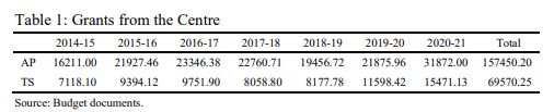
The grants received by AP appears to be more than twice that of TS from above table. But Andhra Pradesh has received the revenue deficit grants alone of
₹59,497 crores. Telangana government didn’t have revenue deficit problem till 2020. Also, as per finance minister’s clarification in Parliament on 10 August 2021, ₹19,427 crores were released in the last seven years? for AP under AP reorganization act (APRA) 2014. However, ₹11,182 Crores of this grant were allocated as part of reimbursement to Polavaram Project expenditure dues demanded by state government for a long time and ₹1750 Crores for backward districts grants which are applicably provided for even Telangana. Thus AP, on the developmental aspect, has not received any advantageous grants compared to Telangana. Despite that, Grants from centre will be taken into consideration for analysis as there is a huge difference in total grants received by both the states in the last seven years.
Fiscal transfers from the central government may mislead results due to no explicit mention of the effectiveness of fiscal policy without central support. Thus, the primary balance will be adjusted for Grants from the centre and the model will be reassessed. Subsidization effects of grants from the centre on primary balance can be estimated through excluding GFC from primary balance and estimating another model for sustainability without central support or sustainability of own fiscal policy of state government. This model can be shown as
𝑚t = ∝0+ 𝛽1𝑑t–1 + 𝛽2𝑅𝑉𝐴𝑅 + 𝛽3𝐸𝑉𝐴𝑅 + 𝑢t …(13)
In the above model, mt refers to adjusted primary balance for Grants from centre taken as the ratio of total receipts. Based on the IBC framework, the government adjusts their taxes to changes in the debt levels, either increasing debt may be shifted by burdening taxes or declining debt levels should reduce the taxes. Thus, debt needs to be correlated with state revenue generation factors. This can be modelled by taking the state’s own revenue as a dependent variable which can be explained by changes in debt, revenue changes and expenditure changes. Taking theoretical backdrop of David Leeper (2011)’s paper, estimation model will be
𝑠𝑜𝑟t = ∝0+ 𝛽1𝑑t–1 + 𝛽2𝐺r + 𝛽3𝐸𝑉𝐴𝑅 + 𝑢t …(14)
Where sort is State own revenue as a percentage of Total Receipts, the variable RVAR of equation 14 is replaced by the growth rate of Total Receipts. These three independent variables are expected to be having positive coefficients.
- Results of the Analysis
Stationarity Tests
Stationarity tests provide for preliminary analysis of the nature of data to be studied. In this study, ADF and PP tests of stationarity are done for UAP, AP, and TS on 18 different variables of state finances. The ADF test has the null hypothesis of unit root present in the series and the PP test revivifies the ADF unit root test results in the null hypothesis. The optimal lag length of each variable under the Schwartz information criterion was taken. For combined Andhra Pradesh all variables are stationary at level except the Debt series. Debt series of UAP are Integrated of order 1, i.e., I (1). Details of the all variables in the study are provided below.

Post bifurcation data variables of both states are taken for similar stationarity tests and found all variables to be stationary except for Debt which is stationary at
first difference as seen from United Andhra Pradesh. Though debt is not stationary at level, Debt as a percentage of Total Receipts is found to be stationary at level. This indicates the series is not so deviating from their constant mean value and this implies that variations in debt can be estimated through cointegration analysis for revenue and expenditure. All the three states have their debt difference as stationary at a level indicating debt sustainability condition satisfied by traditional analysis. But this should be checked with cointegration analysis as stationarity simply can’t imply underlying factors for debt sustainability analysis.
Cointegration Analysis for Debt Sustainability under IBC Approach
The equilibrium relation implied by revenue and expenditure variables of cointegration analysis is the basis for debt sustainability. Unlike previous debt sustainability studies on aggregate level data of state governments, this study provides state-specific relations with adjusted variables such as Total receipts without including debt receipts like ATR, primary balance adjusted for grants from centre as APB.
A few popular cointegration tests are the Engle-Granger cointegration test, Johannsen cointegration test and ARDL bound tests etc., test suitability for data will define the choice of the test by the researcher. For this study, we use Auto- Regressive Distributive Lag (ARDL) bound tests for the cointegration relationship between expenditure and revenue along with the cointegration of debt and primary balance. In case, if revenue and expenditure are not cointegrated, that doesn’t imply debt is completely unsustainable. Unlike other methods, ARDL bound tests are flexible in accommodating variables of different levels of I (0), I (1), i.e., integrated of order zero or one into cointegration analysis. Based on empirical tests, the ARDL method is best suited for small samples. The long-run relationship and short-run dynamics between the variables can be estimated using ARDL bound tests. Error correction mechanism results will explain the speed of adjustability of variables of cointegration. In our study, the adjustment of revenue to changes in expenditure can be explained through ECM. Considering these factors, we are proceeding with ARDL method of cointegration in our analysis.
Distributed lag model implies that the regression function includes unrestricted lag of the regressors. The ARDL (p,q) model specification for our analysis is
𝑇𝐸t = 𝛽1 + 𝛽2𝑇𝑅t + 𝑢t
It implies an estimation model of co-movement relation between TE and TR. If the error term ut is assumed to be stationary and independent of the TR as well as TE and their lags, then models can be estimated through ordinary least squares.
As by Quintos (1995) conditions the coefficient of revenue should be positive and less than or equal to one, should be satisfied for debt sustainability and cointegration relation is not useful when it is not satisfied, i.e., 0 < b ≤ 1 should be
satisfied. In the long-run relation between variables in four models specified for UAP, all are cointegrated in ARDL bound test.
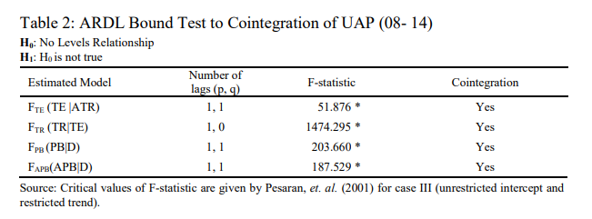
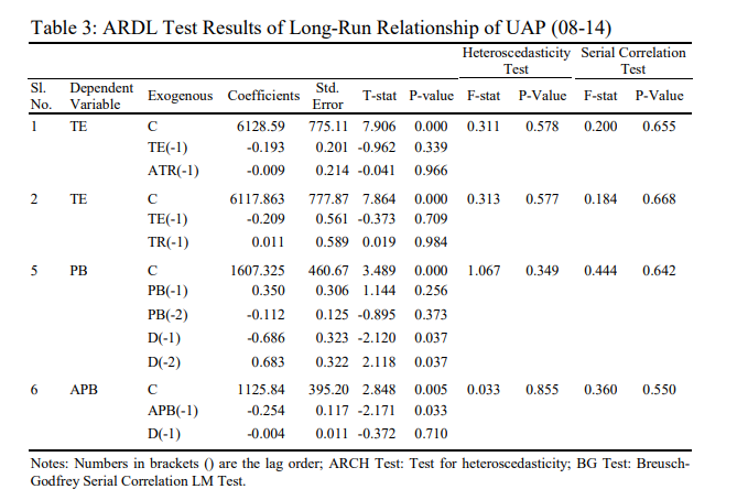
But these cointegration relations cannot guarantee debt sustainability in UAP, because the coefficient value is positive only in TR and TE relation, that too minimal, implying very weak sustainability in UAP
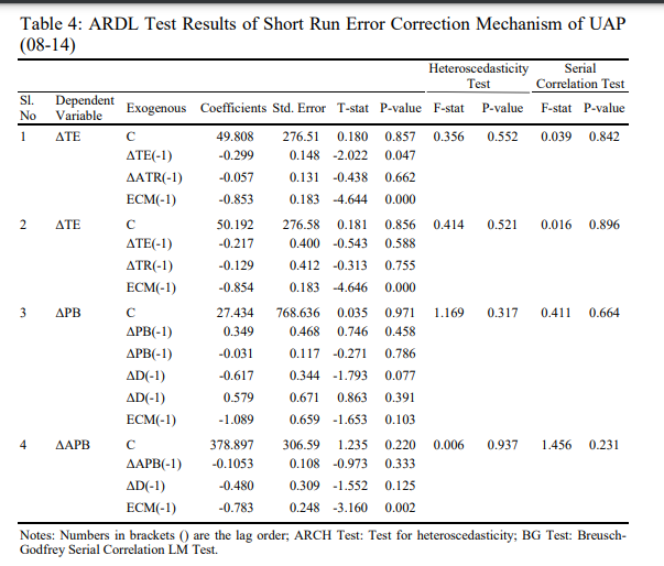
Although the problem of weak sustainability of debt exists for UAP, the Error correction mechanism should push the deviations of revenue from expenditure to sustainability path, the speed at this adjustment happens is explained with 85.4 per cent in UAP. Thus, short-run adjustments of fluctuations in debt are presenting a continual path of weak debt sustainability
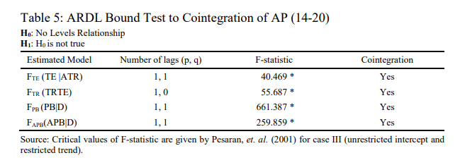
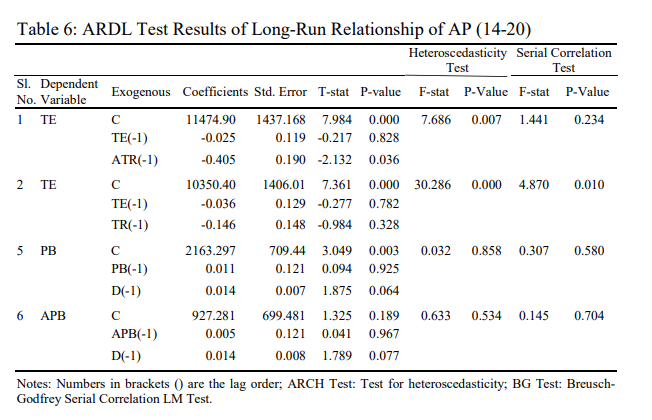
For post bifurcation in Andhra Pradesh, the TR and TE model of cointegration along with all the models did not find any positive coefficient value despite all models being cointegrated. This proves debt as clearly unsustainable post bifurcation for AP. So, the error correction mechanism which is the similar speed of adjustment of UAP, cannot be used for AP series to be adjusted for short-run relation. Even heteroscedasticity and autocorrelation are found to be high, making the models uninterpretable.
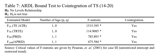
For Telangana, all models satisfied cointegrating conditions along with a positive coefficient value in each model. The coefficient value TE and ATR model is higher among all other models analyzed and also the TE and TR model has a positive coefficient even greater than the UAP model of weak sustainability. The values of coefficients for these models are 0.098 and 0.0368 which are almost close to unsustainability, but we take it as weakly sustainable but better than UAP
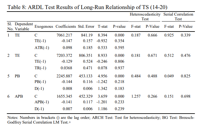
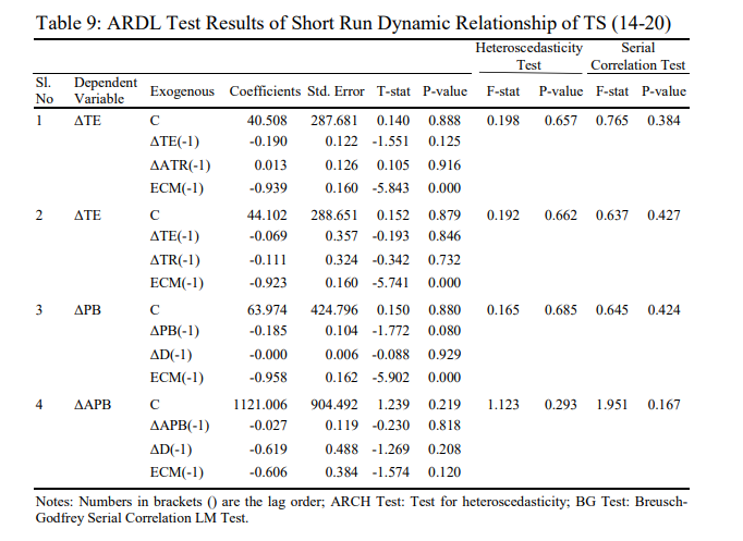
The ECM is also found to be higher compared to the other two states, providing reconfirmation for our interpretation of debt of Telangana to be more sustainable than AP and UAP. A more detailed analysis of structural models designed for fiscal policy response will be analyzed in the next section.
Results of Fiscal Policy Response Models
To understand the debt sustainability of UAP, AP, and TS through fiscal policy response, four different models of regression analysis are used. These models are constructed based on the analysis of debt sustainability by Renjith and Shanmugam (2019). Results of the three states are presented in Tables 10, 11, and 12.
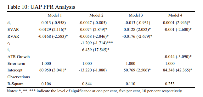
In United Andhra Pradesh, the model 1 values of EVAR and RVAR are statistically significant but negative, which means with the Revenue receipts growth and expenditure growth above their potential, long-run levels have reduced Primary balance. Debt is statistically insignificant, but this model has a low R- square value, making the model invalid for explaining the response function. However, model 1 of AP and TS are statistically significant and the primary balance is positively responding to EVAR in both models. Surprisingly RVAR is again negative, implying the rise in revenue from its potential level is not increasing PB, but reducing it. Since R- square value is comparatively good in TS Model 1, Telangana Debt can be sustainable, but a lower value of coefficient at 0.0087 makes it weakly sustainable.
In model 2, grants from centre and interest payments variables are chosen to explain the changes in PB. Only AP had significant value for debt compared to others but it has less R-square value. AP and TS models failed to get significant relation for the GFC coefficient, which shows the grants from the centre are in no way the determining factor of increasing primary surplus and debt sustainability.
Interest payments turned out to be an important variable explaining the rise in PB, but this relation shows that a rise in IP has increased primary Balance, which is not possible in general.
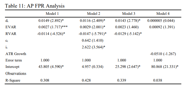
Model 3 explains the adjusted primary balance as a dependent variable which is taken after deducting GFC from PB. But the relevance of significant variables can be compared only for TS because only that has some explainable R-square value compared to others. But subsidization of PB through Grants has a significant effect on states to achieve debt sustainability. For Telangana, it increased the potential to increase primary surplus by a factor of 0.0006, but for Andhra Pradesh, it decreased that potentiality.
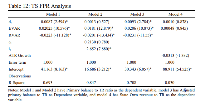
Finally, model four did not have any significant values of debt or expenditure variation in AP and TS. The significant values of UAP are very low, almost negligible with low R-square, making the models not suitable for any debt sustainability when taking SOR as a dependent variable. However, the least explanatory possible, explains that states are Ponzi Financing their Debts.
Almost all the models are showing significant values for EVAR and RVAR, with complete opposite relation of what is generally assumed. It shows that the rise in expenditure above its normal value is raising/increasing the pb rather than reducing it and rise in ATR above its normal value is decreasing the pb rather than increasing it. Since pb is PB-ATR ratio, above results imply that the rise in expenditure is also causing the rise in borrowings and thereby fall in ATR and therefore rise in pb. In RVAR case, the rise in borrowings amounts has the denominator effect of high ATR growth and numerator effect of rising Primary expenditure component of PB, and finally, the fall in pb. Thus, accumulated borrowings are playing a huge role in rising Primary Expenditure, Primary balance is increasing with the rise in expenditure and falling with the rise in Revenue. R- square values are low for all models except Telangana. Telangana explanatory models indicate debt as a Sustainable but weak response to changes in debt.
The monthly data of state government is highly fluctuating with outlier effects on the regressions. Same was found to be true in the monthly data taken for analysis with UAP, AP and TS. There are two major reasons for this. Firstly, all state governments in India try to balance or adjust their budgetary figures in the year end to present budgetary sessions. Secondly, uncertain circumstances affect the state finances. For example, bifurcation movements in 2011 in UAP, the leadership changes due to political turmoil, financial crisis 2008, election years, sudden changes in the fiscal policies (either expenditure side or revenue side or both). Suppressing these outliers has improved the R-square value and significance of the models.
To validate the results, the diagnostics tests such as Correlogram, Breusch- Godfrey Serial correlation LM test, Breusch-Pagan-Godfrey Heteroskedasticity test, ARCH heteroskedasticity test, Histograms, Ramsey RESET test for specification errors, CUSUM and CUSUM squares test for stability, Shapiro-Wilk Normality test, Kolmogorov-Smirnov Normality test are done for all the 12 models of cointegration in IBC approach and 12 regression models of FPR approach. The problem of outliers has been a recurrent problem in stability tests and normality tests. Good results are found in all the tests. Suppressing the outliers have resulted in resolving the problems in stability and normality tests. But as monthly outliers are an intrinsic part of data, they cannot be removed for fitting of the model. Even if the disturbance term is not normally distributed, OLS estimators are normally distributed under the assumption of homoskedasticity (which is satisfied in this study). Further study is recommended for identifying the outlier effects and restricting them with including filtered significant variables in the regression models.
II Conclusion
In this paper, two approaches are discussed on DSA of AP, TS, and UAP. Theoretical construction of these models, along with their application for DSA of AP, TS and UAP are examined. IBC for DSA involves stationarity and Cointegration analysis, the results of the analysis show the debt is unsustainable in AP, but UAP and TS had Sustainability at low levels, making the long-run risk for solvency. On the other hand, the FPR approach is used with a framework implemented for four distinct models for explaining debt sustainability. All the models failed to prove debt sustainability in AP and UAP but provided evidence for weak sustainability in TS in all these models. The results indicate Primary balance for AP and TS is nowhere near sustainability, whereas TS is better compared to those both. However, the latter has long-term problems with sustainability of debt and cointegration revenue and expenditures.
IBC and FPR approaches present DSA through econometric estimation models and their properties. The difference series of outstanding debt stocks of UAP, AP, and TS are stationary at level, implying debt paths will equilibrate primary surpluses and debt stock at some point based on the IBC approach. The results of the ADF test are backed by similar results in PP stationary test. All the cointegration results pinpointed that the relationship between revenue and expenditure exists, but positive coefficient values are found only for TS and UAP. Among these, TS has a slightly stronger relation than UAP, but both are weakly sustainable under the IBC hypothesis. Even ECM adjustments are better in TS compared to the other two states.
Response of state governments to rising debt levels is important and is traditionally estimated through the response of PB to Debt Stock. All the models constructed for AP and UAP are found to be indecipherable for catching policy responsiveness of these states to debt variations. TS has positive PB changes with debt increase but it is a very weak relation. Even UAP has a possible sustainability case when interpreted, but that is very less sustainable of debt relative to TS. AP needs to ask the centre for rightful grants under APRA 2014 and assistance in other forms such as central support projects in the form of capital outlay. Because of the bifurcation disadvantages, the initial phase of revenue deficit path is inevitable. AP needs to focus more on stability in generating the state’s own revenue. The expenditure of all three states is positively affecting primary balance, which needs further analysis through more apt DSA model construction.
References
Barro, R.J. (1979), On the Determination of the Public Debt, Journal of Political Economy, 87(5): 941-970.
Bohn, H. (1995), The Sustainability of Budget Deficits in a Stochastic Economy, Journal of Money, Credit and Banking, 27(1): 257-271.
———- (1998), The Behavior of U.S Public Debt and Deficits, Quarterly Journal of Economics,
113(3): 949-963.
Bohn, H. (2005), The Sustainability of Fiscal policy in the United States, Cesifo Working Paper 1446.
———- (2007), Are Stationarity and Cointegration Restrictions Really Necessary for the Intertemporal Budget constraint? Journal of Monetary Economics, 54(7): 1837-1847.
Buiter, W.H. (1983), Theory of Optimum Deficits and Debt, NBER working papers 1232.
———- (1985, november), A Guide to Public Sector Debt and Deficits, Discussion Papers, 501. Buiter, W.H., and U.R. Patel (1992), Debt, Deficits and Inflation: An Application to the Public
Finances of India, Journal of Public Economics, 47(2): 171-205.
Davig, T. and E.M. Leeper (2011), Monetary – Fiscal Policy Interactions and Fiscal Stimulas.
European Economic Review, 55(2): 211-227, doi:10.1016/j.euroecorev.2010.04.004
Frickle, B. and A. Greiner (2011), Debt Sustainability in Selected Euro Area Countries: Empirical Evidence Estimating Time-varying Parameters, Studies in Nonlinear Dynamics and Econometrics, 15(3): 1-21.
Hakkio, C.S. and M. Rush (1986, December), Co-integration and the Government’s Budget Deficit,
Research Working Paper, No. 86-12.
———- (1991), Is the Budget Deficit ‘Too Large’? Economic Enquiry, 29(3): 429-445.
Hamilton, J.D., and M. Flavin (1986), On the Limitation of Government Borrowing: A Framework for Empirical Testing, American Economic Review, 76(4): 808-819.
Mohanty, R. and S. Panda (2019, January), How Does Public Debt Affect the Indian Macro- Economy? A Structural VAR Approach, NIPFP Working Paper No.250, New Delhi.
Pradhan, K. (2014), Is India’s Public Debt Sustainable? South Asian Journal of Macro economics and Public Finance, 3(2): 241-266.
Quintos, C.E. (1995, October), Sustainability of Deficit Process with Structural Shifts, Journal of Business and Economic Statistics, 13(4): 409-417, Retrieved from https://www.jstor.org/stable/1392386
RBI (2019, September), State Finances: A Study of State Budets of 2019-20, RBI.
Renjith, P.S. and K.R. Shanmugam (2019), Dynamics of Public Debt Sustainability in Major Indian States, Journal of Asia Pacific Economy, doi:10.1080/13547860.2019.1668138
Shastri, S. and M. Sahrawat (2012), Fiscal Sustainability in India: An Empirical Assessment, Journal of Economic Policy and Research, 10(1): 97-112.
Trehan, B. and C.E. Walsh (1988, September), Common Trends, the Government Budget Constraint and Revenue Smoothing, Journal of Economic Dynamics and Control, 12(2-3): 425-444, doi:https://doi.org/10.1016/0165-1889(88)90048-6
Wilcox, D.W. (1989, August), The Sustainability of Government Deficits: Implications of Present- Vlue Borrowing Constraint, Journal of Money, Credit and Banking, 21(3): 291-306.